One of the simplest models of mid-latitude dynamics is Phillips’ two-layer quasi-geostrophic (QG) model on a \(\beta\) plane. This consists of two layers of constant density, with the top layer lighter than the bottom layer, whose interface is relaxed to some equilibrium slope (which represents the tropics receiving more solar radiation than high latitudes). Surface friction is also present in the lower layer:

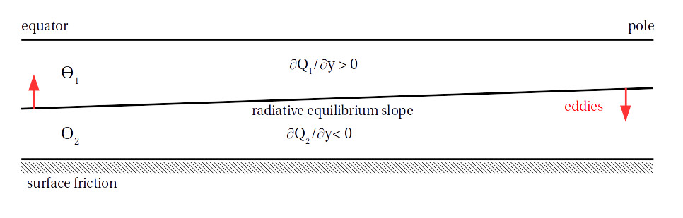
\(\theta\) is potential temperature and \(Q\) is the zonal-mean potential vorticity, defined below. The non-dimensionalized equations for the two layers are: $$ \frac{\partial q_k}{\partial t} + J(\psi_k, q_k) = -\frac{1}{\tau_d}(-1)^k (\psi_1 - \psi_2 - \psi_R ) - \frac{1}{\tau_f}\delta_{k2}\nabla^2 \psi_k (+ hyperdiffusion), $$ where \(q_k = \nabla^2 \psi_k + (-1)^k (\psi_1 - \psi_2) + \beta y\) is the potential vorticity (PV) in each layer, with \(\psi_k\) the streamfunction in each layer and \(\beta\) the meridional gradient of the Coriolis parameter. \(k\) = 1 for the top layer and 2 for the bottom layer, and the \(\delta\)-function indicates that the friction only acts in the lower layer. \(\psi_R\) is the equilibrium slope which the interface is relaxed to, and is chosen to make the system baroclinically unstable. The way to think about the dynamics is that eddies try to flatten out the interface by transporting heat polewards, fighting against the radiative relaxation

This system was used by Phillips in 1956 as the basis for the first numerical weather model, and since then we’ve learned a lot about the atmosphere by studying the two-layer model because, despite its simplicity, it captures the main features of the mid-latitude circulation that we care about, like annular modes and other behaviors of eddy-driven jets. (Similar systems are used to study jets in the ocean and on other planets).

The Two Climates of the Model

An important feature of the model’s climate (and of Earth's troposphere) is that the zonal-mean PV gradient in the upper layer is larger in magnitude than the PV gradient in the lower layer: $$ \frac{dQ_1}{dy} = \beta - \frac{d^2 U_1 }{dy^2} + (U_1 - U_2), \\ \frac{dQ_2}{dy} = \beta - \frac{d^2 U_2 }{dy^2} - (U_1 - U_2), $$ where \(U\) is the zonal-mean zonal wind and the main balance is between \(\beta\) and the vertical wind shear \((\beta + (U_1 - U_2) > \beta - (U_1 - U_2))\). This means that eddies can propagate further from their source in the upper layer than in the lower layer, which makes the dynamics of the upper layer more linear. In the lower layer the waves essentially just form and break (non-linearly) in place (see here for more on lower layer eddies).

How could we switch this, to make the PV gradient in the lower layer larger? One way is to reverse the temperature gradient so that the “pole” gets more sun than the “tropics”. This would be the case on a planet with high obliquity, and in the two-layer model is done by reversing the sign of \(\psi_R\): $$ \frac{\partial q_k}{\partial t} + J(\psi_k, q_k) = -\frac{1}{\tau_d}(-1)^k (\psi_1 - \psi_2 + \psi_R ) - \frac{1}{\tau_f}\delta_{k2}\nabla^2 \psi_k. $$ The vertical wind shear is then negative \((U_1 - U_2 < 0)\) and the PV gradient is larger in the lower layer.

Another way to make the PV gradient larger in the lower layer is to take the original set-up and change the sign of \(\beta\). This could happen with a strong, negative topographic \(\beta\), but otherwise you have to imagine a planet that's wider at the poles than at the equator (like an inverted cone).

Everything stays the same except that the PV is now \(q_k = \nabla^2 \psi_k + (-1)^k (\psi_1 - \psi_2) - \beta y\). If we then make the co-ordinate transform \(x, y → -x, -y\), we get exactly the same system as when reversing the temperature gradient: $$ \frac{\partial q_k}{\partial t} + J(\psi_k, q_k) = -\frac{1}{\tau_d}(-1)^k (\psi_1 - \psi_2 + \psi_R ) - \frac{1}{\tau_f}\delta_{k2}\nabla^2 \psi_k, \\ q_k = \nabla^2 \psi_k + (-1)^k (\psi_1 - \psi_2) + \beta y. $$

So changing the sign of \(\beta\) (i.e., the sign of the rotation gradient) and making the co-ordinate transform \(x, y → -x, -y\) is exactly the same as reversing the temperature gradient. A final way of getting to this is to move the friction to the upper layer: $$ \frac{\partial q_k}{\partial t} + J(\psi_k, q_k) = -\frac{1}{\tau_d}(-1)^k (\psi_1 - \psi_2 - \psi_R ) - \frac{1}{\tau_f}\delta_{k1}\nabla^2 \psi_k, $$ and then switch the layers, i.e., make the co-ordinate transform \(z → -z\): $$ \frac{\partial q_k}{\partial t} + J(\psi_k, q_k) = -\frac{1}{\tau_d}(-1)^k (\psi_2 - \psi_1 - \psi_R ) - \frac{1}{\tau_f}\delta_{k2}\nabla^2 \psi_k. $$

We could summarize all this by saying that the two-layer model has two climate: the Earth-like climate 1, and climate 2, which is like a planet with a reversed temperature gradient. We can go from climate 1 to climate 2 by making one of the perturbations discussed above, and can go back by adding another perturbation:

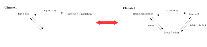
The key difference between the two climates is that in climate 1 the friction is in the layer with the smaller PV gradient and in climate 2 the friction is in the layer with the larger PV gradient. This affects the eddy fluxes, but I'm not going to go into that here.

Simulating the Climates

Here’s what the zonal-mean winds in the two layers look like in simulations of these climates with Earth-like parameters:

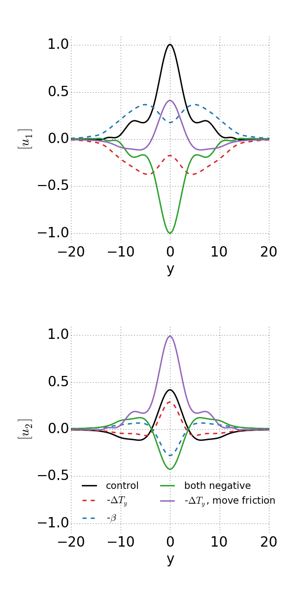
In the reversed temperature gradient case there are two strong easterly jets in the upper troposphere, while the winds in the lower troposphere are pretty similar to the control case, because they still have to balance the vertically-integrated eddy momentum flux divergence.

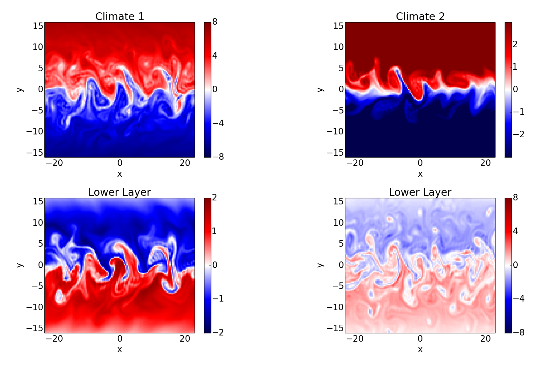
And for reference, here are snapshots of the PV in both layers of an Earth-like simulation and a simulation with the temperature gradient reversed:

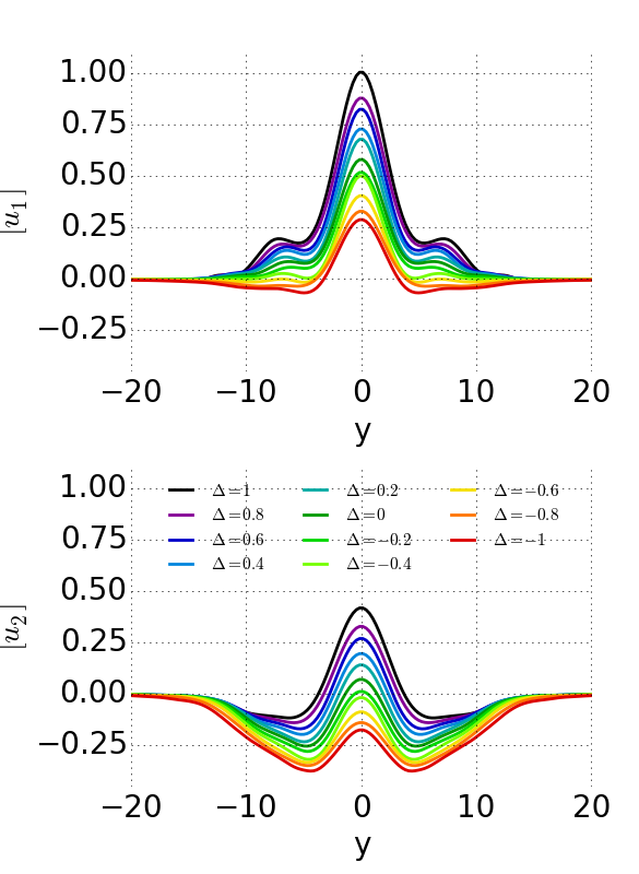
Taking things further, the two climate are actually end-members of a continuum of climates; it is really the ratio of the friction in the two layers which matters. We can define a quantity \(\Delta\), which is equal to the friction in layer 2 minus the friction in layer 1, divided by the friction in layer 2: \(\Delta = (\tau_{f, 2} - \tau_{f, 1} ) / \tau_{f, 2}\), and then go smoothly from climate 1 to climate 2 by varying \(\Delta\) from 1 to -1:

Finally, for some more realistic examples, here are the zonal-mean winds (black contours) and eddy momentum fluxes (colored contours) from some simulations with the GFDL dry dynamical core, forced with Held-Suarez physics, of an Earth-like case (top), a case with a reversed temperature gradient (middle) and a case with a reversed temperature gradient and friction in the upper troposphere (bottom):

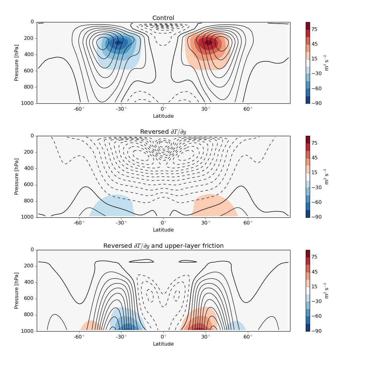
The spherical geometry and the presence of a stratosphere mean things aren’t exact anymore, but qualitatively these are similar to the corresponding two-layer simulations.

Some Implications

I've already mentioned some situations in which climate 2 would be relevant, like a planet with high obliquity and a situation with a strong negative topographic \(\beta\) effect. The flow underneath an ice shelf might also be like climate 2 if the water feels a strong frictional force from the ice.

Besides these special cases, I think the more interesting point is that these results highlight the symmetries of the 2-layer model, which mean that its climate is defined by the position of the friction relative to the PV gradient. This is really the only degree of freedom in the model; we can change parameter values, but as long as the friction is in the layer with the smaller PV gradient the climate is fundamentally "Earth-like".

(Email me if you want code for any of the simulations).