The best datasets we have for constraining Earth's climate sensitivity are the historical records of temperature and TOA radiative fluxes. Intuitively, it seems like we should be able to use these to say something about Earth's climate sensitivity, but this turns out to be pretty subtle.

One issue which has gotten attention recently is that inferred climate sensitivity changes over time:

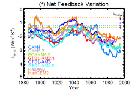
(From Andrews et al. (2018); \(\lambda\)is calculated by regressing \(R\)against \(T\)over sliding 30 year windows for simulations of the historical record with eight different climate models.)

The climate feedback parameter \(\lambda\) was small between about 1920 and 1960 (implying a high climate sensitivity) and has been increasing since then (implying a lower sensitivity). To calculate this, an assumption is made about the forcing \((F)\) and then the global-mean surface temperature \((T)\) is regressed against the net TOA flux \((R)\), using \(R = F - \lambda T\). Alternatively, you can also calculate \(\lambda\) as the derivative \(\partial R / \partial T\). Either way, observations and models give a consistent picture of \(\lambda\) changing over the 20th century.

Explaining this with the Pattern Effect

One way to explain this is through the "pattern effect": the feedback at a particular time is partly determined by the pattern of warming. So the strength of \(\lambda\) changes over time as anomalous SST patterns change over time.

To see how this works, take a two box model of Earth's climate, with energy transport parameterized based on the temperature difference between the two boxes. You can think of these as a high latitude box and a low latitude box, or an east Pacific box and a west Pacific box,... The TOA radiation budget for this system can be written as $$ R_1(t) = F_1(t) + F_{r, 1}(t) - \lambda_1 T_1(t) - c(T_1(t) - T_2(t)),\\ R_2(t) = F_2(t) + F_{r, 2}(t) - \lambda_2 T_2(t) + c(T_1(t) - T_2(t)), $$

where \(T_i\) is the temperature in box \(i\), \(\lambda_i\) is the "local" radiative feedback in box \(i\), \(F_i\) is the CO\(_2\)forcing in box \(i\), \(F_{r, i}\) is the non-CO\(_2\)forcing in box \(i\) and \(c\) is the rate of anomalous heat transport between the two boxes.

These can then be divided up into components due to the CO\(_2\) forcing (subscript \(F\)) and residuals, which include the internal variability, aerosols, etc. (subscript \(r\)) $$ R_{F, 1}(t) + R_{r, 1}(t) = F_1(t) - \lambda_1 (T_{F, 1}(t) + T_{r, 1}(t)) - c(T_{F, 1}(t) + T_{r, 1}(t) - T_{F, 2}(t) - T_{r, 2}(t)), \\ R_{F, 2}(t) + R_{r, 2}(t) = F_2(t) - \lambda_2 (T_{F, 2}(t) + T_{r, 2}(t)) + c(T_{F, 1}(t) + T_{r, 1}(t) - T_{F, 2}(t) - T_{r, 2}(t)), $$

For simplicity, I'm assuming that the \(\lambda\)'s and \(c\) don't change over time, and also that they take the same values for the forced components as for the residuals. To make things even easier, I'm also taking out any residual forcing, like aerosols, so there's just internal variability.

In this system, changes in the climate sensitivity are entirely due to changes in the pattern of warming, since the \(\lambda\)'s are constant over time and don't change for different forcings or for internal variability. The global-mean feedback parameter in this system at a particular time \(t\)is $$ \lambda_g(t) = \sum\lambda_i T_{F, i}(t) / \sum T_{F, i}(t) $$

The global-mean feedback depends on the warming in each box and on the local feedback of each box. So, even if nothing else happens, \(\lambda_g\) changes over time as \(T_{F, 1}\) and \(T_{F, 2}\) change. If box 1 has a high sensitivity (small \(\lambda_1\)) and box 2 has a low sensitivity (large \(\lambda_2\)), but for some reason box 2 warms up faster than box 1, then the observed climate sensitivity will increase over time as the warming in box 1 catches up. (Differences in ocean heat uptake could cause these different rates of warming.).

Adding in the residual, the inferred feedback parameter becomes $$ \lambda_{g, in}(t) = \sum \lambda_i (T_{F, i}(t) + T_{r, i}(t)) / \sum (T_{F, i}(t) + T_{r, i}(t)). $$

The residual temperature patterns -- here just made up of internal variability -- can cause large changes in the inferred climate sensitivity, and have to be taken out to accurately estimate \(\lambda_g\).

In summary, although the local feedbacks are constant, the inferred global-mean feedback parameter changes over time both because the pattern of the forced response changes and because of internal variability. In equilibrium, the global-mean feedback is $$ \lambda_{e, g} = \sum\lambda_i T_{F, i, e} / \sum T_{F, i, e}. $$

where the subscript \(e\) denotes an equilibrium quantity so the temperatures don't change over time anymore. This is what we're really after, but even if we knew the \(\lambda_i\)s -- if we knew all the local feedbacks -- we still wouldn't know the equilibrium climate sensitivity because we wouldn't know the equilibrated temperature pattern, the \(T_{F, i, e}\)s.

In this simple model, the pattern effect makes it hard to estimate Earth's sensitivity from the historical record, as the inferred global-mean feedback parameter changes over time both because the pattern of the forced response changes and because of internal variability. In the real world, there's also the residual forcings of aerosols, volcanoes, etc.; the possibility that the local feedbacks change over time; the possibility of non-local feedbacks; and ocean heat uptake, which I've mostly ignored here. Going back to the data, the changing inferred climate sensitivity over the historical record is the result of some combination of internal variability, changing patterns of the forced response and non-CO\(_2\) forcings. Untangling these isn't easy, and Andrews et al. attribute the decreasing sensitivity over the historical record to changing SST patterns that result in more negative global-mean cloud and clear-sky longwave feedbacks. The next challenge is figuring out why SSTs changed in this way.