Someone asked me recently about the difference between weather and climate. When do we call it “weather” and when is it “climate”? And how can we predict the climate 10 or 100 years from now, when it’s so hard to predict the weather a week from now?
As part of this conversation it came up that, even with a perfect weather model, tiny errors in the observed state of the atmosphere mean that we’d only be able to get accurate forecasts for up to about two weeks. For longer lead-times the model would lose all skill, until we got to seasonal time-scales: we can safely predict that summer will be warmer than winter.
The reason for this is that errors – either problems with the model or with the observations used to initialize the model – grow faster at smaller scales than they do at larger scales. We can quantify this with doubling times: error takes much longer to grow from some scale \(x\) to \(2x\) than from \(x/2\) to \(x\). Faster doubling times at small scales put a limit on the atmosphere’s predictability, since at a certain point the improvements from increasing resolution and improving data quality are negligible.
As an example, imagine we had a weather model and observations that were accurate down to 10km resolution, and we said the model became unusable once the errors reached a scale of 100km. If we improved the resolution down to 5km, any initial errors would grow so quickly that we’d only get a small increase in the forecast lead time compared to the 10km model and observations:
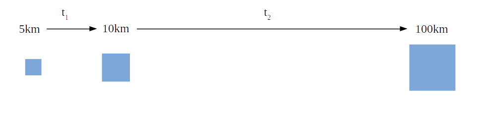
We'd get even smaller gains from improving the resolution down to 2.5km, 1.25km, etc.
The “finite” predictability of the atmosphere, caused by the rapid doubling times at small scales, was first shown by Ed Lorenz in a 1969 paper. Plugging in some numbers, Lorenz did a back-of-the-envelope calculation to estimate that the predictability of the atmosphere is limited to about 2 weeks at most.
A Problem with Lorenz's Theory
In 2008, Rotunno and Snyder showed that there was a problem with Lorenz’s derivation. As part of the derivation, Lorenz had to assume something about the kinetic energy (KE) spectrum of atmospheric turbulence. The KE spectrum is the amount of kinetic energy contained at each wavenumber \(k\) (the inverse wavelength) of the turbulence and is typically assumed to follow a power law: $$ E \sim k^{-p} $$ Lorenz was working with 2D turbulence (the aspect ratio of the atmosphere is so large that we can treat it as being ~2D) and assumed \(p = -5/3\): $$ E_L \sim k^{-5/3} $$ following Kolmogorov’s classic result for 3D turbulence. Lorenz’s derivation relies on this 5/3 power to show that errors grow faster at smaller scales. But for 2D turbulence \(p\) is actually equal to 3: $$ E_{2D} \sim k^{-3} $$ (note: the \(k^{-3}\) scaling was discovered around the same time as Lorenz did his calculations).
Substituting \(p = -3\) into the derivation gives “infinite” predictability: the rate of error growth is independent of scale, so that going from a 10km model to a 5km model increases the lead time by a factor of 2. If \(E\) is proportional to a higher power than 3, errors take longer to grow at small scales than at large scales and using a better model gives a big increase in lead time.
To see the difference, Rotunno and Snyder compared the growth of error energy for \(k^-5/3\) and \(k^-3\) spectra:
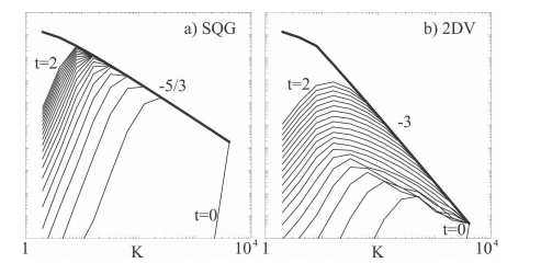
(Figure 1 from Rotunno and Snyder, 2008.)
In the \(k^{-3}\) case the error growth is roughly constant in time in wavenumber space, whereas for \(k^{-5/3}\) the error grows much faster at high wavenumbers than at low wavenumbers (large scales).
A Problem with Lorenz's Theory
To get back to the 2 week predictability barrier, Rotunno and Snyder noted that observations show that on scales smaller than about 1000km, the atmosphere roughly follows \(k^{-5/3}\) scaling:
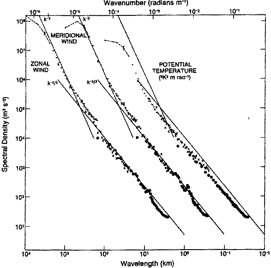
(Figure 1 from Tung and Orlando (2003), note that the meridional wind and potential temperature data have been offset by a constant factor so they can be plotted on the same figure.)
It’s thought that in this regime the atmosphere is best represented by surface quasi-geostrophic (SQG) turbulence, which is a kind of intermediate between 2D and 3D turbulence. See here for more. The kinetic energy spectrum for SQG has a \(k^{-5/3}\) scaling and so there is a finite predictability barrier.
Error Growth as Turbulent Dispersion
The derivations by Lorenz and Rotunno and Snyder are long and technical, so it’s hard to get an intuitive feel for the difference between these different kinds of turbulence. Instead, I like to think about error growth as being like the dispersion of a passive tracer in a fluid: imagine two small patches of “error” in the atmosphere, how quickly do these move apart?
There is some classic literature on turbulent dispersion, going back to (at least) Richardson (1926), who derived the “4/3” law. If we model dispersion as a diffusive process, then a scaling for the diffusivity is: $$ D \sim \sqrt{E l} $$ where \(l\) is a length scale (the separation between the error patches) and \(E\) is the kinetic energy density (units of energy/unit wavenumber or energy \(\times\) length). Substituting in \(E \sim k^{-5/3} = l^{5/3}\) then gives $$ D \sim l^{4/3}. $$ We can get a characteristic spreading time-scale by dividing \(l^2\) by \(D\): $$ t \sim l^2 / D \sim l^{2/3} $$ So the characteristic spreading time-scale is longer for larger scales or distances (though the dependence is less than linear). Substituting the \(k^{-3}\) (\(l^3\)) spectrum instead gives $$ D \sim \sqrt{E_{2D} l} \sim \sqrt{l^4} = l^2 $$ and hence $$ t \sim l^2 / D \sim l^0 $$
The spreading time-scale is now independent of length-scale, just as Rotunno and Snyder found in their formal derivation. You can also see that if \(p\) is greater than 3 the error spreading time is longer for smaller scales. (Note that an issue with what I’ve done here is it treats the error as a passive tracer – is it better to treat it as an active tracer?).
So one way of thinking about predictability is that it depends on how quickly errors diffuse to larger scales. In 2D turbulence the diffusivity grows as distance \(l^2\), which is fast enough for the doubling time to be roughly constant as a function of scale, but for 3D turbulence and SQG, which are a better match for the observed atmosphere, the diffusivity grows more slowly, proportional to \(l^{4/3}\), and so the doubling time increases for larger scales.
(Thanks to Chris Lutsko for feedback on an earlier version of this post.)