Solar geoengineering, or solar radiation management (SRM), is often put forward as a way of counteracting the global warming effects of increased CO\(_2\) concentrations. The idea is that by reducing the amount of incoming solar radiation reaching Earth's surface, we can (partially) compensate for some of the extra heat trapped by higher CO\(_2\) concentrations. The main proposed way of doing this is injecting aerosols (small particles) into the stratosphere, where they would reflect sunlight back to space (wikipedia page here).

There are a lot of questions, political and scientific, about SRM. A question I've been thinking about is how to optimize SRM. That is: what is the best way of implementing SRM to counteract the effects of global warming?

One option is to focus on maintaining the equator-to-pole temperature gradient. This is one of the key features of the climate system, and controls many other aspects of the climate. For instance, the speed and position of the mid-latitude jet are largely set by the temperature gradient. Under global warming we expect the equator-to-pole temperature gradient to weaken, because higher latitudes warm faster than low latitudes. This would cause the jet to slow down, and we also expect the jet to shift polewards, though the jury is still out on why exactly. Both of these changes would have major consequences for climates at mid- and higher latitudes.

Many SRM studies consider SRM implementations in which the incoming solar radiation is reduced by 1% at all latitudes (e.g., Irvine et al. from earlier this year; let's ignore the engineering question of how to achieve this). However, in the annual-mean the tropics receive more sunlight than the high latitudes (see panel a of the figure below), so reducing the solar radiation by the same fraction at all latitudes results in a much larger cooling of the low latitudes than of the high latitudes, and the equator-to-pole temperature gradient still weakens. Alternatively, we could decrease the incoming radiation by the same amount at all latitudes, which would lead to a more uniform cooling, maintaining the equator-to-pole temperature gradient.

To test these two options, I did some calculations with a simple moist energy balance model (EBM -- see Merlis and Henry for details). This consists of a single equation: $$ C \frac{\partial T (\phi)}{\partial t} = \frac{1}{4}QS(\phi)a(\phi) - (A + BT(\phi)) - \nabla\cdot\mathbf{H}(\phi) + F , $$ where \(C\) is the heat capacity of the ocean mixed-layer, \(T\) is temperature, \(\phi\) is latitude, \(t\) is time, \(\frac{1}{4}QS(\phi)a(\phi)\) is the incoming radiation as a function of latitude, \(A + BT(\phi)\) approximates the radiative feedbacks, \(\nabla\cdot\mathbf{H}(\phi)\) is the diffusion of moist static energy \((h)\) and \(F\) is some radiative forcing, like that due to increasing CO\(_2\) concentrations. I've used the same parameter values as Merlis and Henry, and the script for the calculations is here.

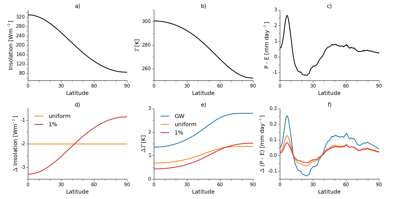
As a control, I integrated the moist EBM to equilibrium with \(F = 0\), giving a surface temperature profile that compares reasonably well with what we see on Earth (panel b of the figure). The temperature response to a uniform forcing of 4Wm\(^{-2}\) is then shown by the blue curve in panel e. This also looks like a typical global warming response, with the warming amplified at high latitudes. I then did two more experiments with the solar constant (\(Q\)) reduced uniformly by 2Wm\(^{-2}\) and with \(Q\) reduced by 1% (see panel d for the changes in insolation).

The temperature responses in the two SRM cases (orange and red lines in bottom left panel) show clearly that the equator-to-pole temperature gradient increases more when \(Q\) is reduced by 1% compared to a uniform reduction in \(Q\).

But even with a uniform reduction, there is greater warming at high latitudes. The reason for this is that the moist static energy, \(h = c_pT + L q_v\), depends on moisture as well as temperature. In a warmer world moisture increases faster at low latitudes than at high latitudes, following the Clausius-Clapeyron relation, and \(h\) does as well. Since the MSE gradient increases, more MSE is diffused to higher latitudes, causing them to warm up more. So to really maintain the equator-to-pole temperature gradient we would actually want to reduce the incoming solar radiation more at high latitudes than at low latitudes.

This is an idealized calulation, but Ban-Weiss and Caldeira (2010) looked into this problem using the NCAR CAM3.1 atmospheric model, trying to optimize the sulphate aerosol distribution so as to minimize the perturbation to surface temperatures. Just like with the EBM, they found that a greater reduction of solar radiation at high latitudes is needed. Interestingly, they also tried to optimize the aerosol distribution to reduce the perturbation to the hydrologic cycle, which they defined as precipitation minus evaporation (P - E). They found it harder to minimize the perturbation to P - E, and also found that a more uniform distribution of aerosols was needed, corresponding more closely to the 1% case.

Can we understand this using the moist EBM? Neglecting changes in moisture transports, the change in P - E can be approximated as: $$ \Delta (P - E) = \alpha\Delta T(P - E) $$ where \(\alpha \sim\)7%K\(^{-1}\) (this comes from Held and Soden (2006)). So the changes are large where the climatological P - E is large ("wet get wetter, dry get drier"). Panel c of the Figure shows the climatological P - E in the Northern Hemisphere, calculated from the MERRA reanalysis dataset. This is largest in the tropics and subtropics, then tapers off at higher latitudes. Panel f shows the responses of P - E for each of the three moist EBM calculations, with the largest changes in the tropics and subtropics, as expected. Both of the SRM schemes reduce the change in P - E compared to the global-warming only calculation, and the P - E change is reduced more in the 1% case than in the uniform case. The reason for this is that the 1% run has a larger temperature change at low latitudes, where the change in P - E is largest. At higher latitudes the two cases are very similar, since the change in P - E is anyways small.

So there seems to be a trade-off between minimizing the temperature perturbation and minimizing the perturbations to the hydrologic cycle. These roughly correspond to an emphasis on cooling high latitudes more versus cooling the tropics more. And of course this is all an annual-mean and zonal-mean picture. We could also worry about regional climates, like minimizing the disruption of the monsoons, and about how these results would change over the seasonal cycle. Even before thinking about the engineering question of how to maintain these aerosol distributions, this is a tricky problem.