Atmospheric stationary waves are planetary-scale waves that are roughly stationary over the course of a season. So the winter stationary wave pattern is different from the summer stationary wave pattern. Stationary waves are excited by topography (large-scale mountains), diabatic heating (e.g., due to convection) and by transient eddy heat and momentum fluxes. These waves transport heat, moisture and momentum around the climate system, and play an important role in regional climates. For example, in a classic paper, Rodwell and Hoskins (1996) showed that a stationary wave excited by convection over India during the monsoon season is partly responsible for the intense dryness of the Sahara. If we want to understand regional climate change (including changes in temperature and precipitation extremes), we have to understand how stationary waves change.

People often separate out the “direct” and “indirect” effects of increasing CO\(_2\) concentrations. The direct effect refers to the system’s response to the radiative forcing from increased CO\(_2\), independent of changes in sea surface temperatures (SSTs), i.e., to the extra atmospheric heating from higher CO\(_2\). The indirect effect is the response to the warmer SSTs, independent of the radiative forcing. In both cases, land temperatures are allowed to evolve freely. The idea behind this decomposition is that the climate system adjusts quickly to the direct effect, whereas the oceans take a while to warm up. The total response is usually pretty close to the linear addition of the responses to the two effects, and you can also think of this as separating out the “fast” response and the “slow” response.

Surprisingly, when doing this kind of decomposition for summer stationary waves, the direct and indirect effects produce the opposite responses, so that the net effect is the residual of a “tug of war”:

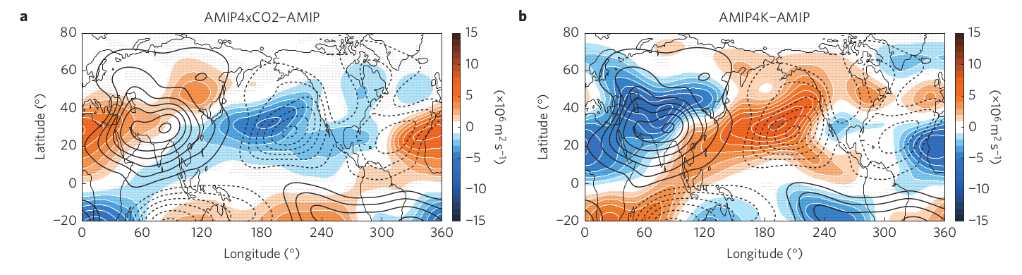
(Adapted from Figure 2 of Shaw and Voigt (2015). The shading shows the responses of the 200hPa stationary eddy streamfunction and the contours show the climatological 200hPa stationary eddy streamfunction.)

How can we understand this? One explanation points to land-sea differences. The idea is that when only the radiative forcing is applied the land warms up but the SSTs are fixed, and so the land-sea moist static energy (MSE) gradient increases. Under a quasi-equilibrium view, the strongest convection occurs where the MSE gradient is largest (see section 5 here for background theory), and if the land-sea MSE gradient increases we should expect stationary waves excited by convection (which dominate the summer stationary wave pattern) to strengthen. Conversely, increasing SSTs reduces the land-sea contrast, weakening these waves.

I buy the first part – the increasing land-sea contrast under the direct effect, but the second part doesn’t make as much sense. The land is still free to warm up when the SSTs are increased, so why should the land-sea contrast decrease?

Baker et al. (2019) have some plots of the changes in \(\theta_E\) (~MSE) in a GHG simulation (+100ppm) and an SST simulation (2005-2015 averaged SSTs), relative to a control (pre-industrial) simulation:

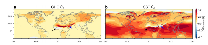
(Figure 8 from Baker et al. (2019). Differences in \(\theta_E\) between a +100ppm CO\(_2\) simulation and a control simulation (a) and between a simulation with 2005-2015 averaged SSTs and the control simulation.)

In the GHG simulation there are some notable changes in the land-sea MSE gradients, particularly where they’ve put arrows, but the land-sea contrast actually decreases in some places, especially off the west coast of Africa. There are some land-sea changes in the SST simulation, but to me the most noticeable gradient is the meridional gradient: the largest \(\theta_E\) changes are in the deep tropics, with weaker changes in the subtropics and higher latitudes.

Deser and Phillips (2009) give a different explanation for the opposing impacts on stationary waves. CO\(_2\) forcing on its own stabilizes the atmosphere, suppressing convection, while warming SSTs increases the atmosphere’s moisture content, which provides more energy for convection. So tropical forcing of stationary waves strengthens in response to the indirect effect but weakens in response to the direct effect.

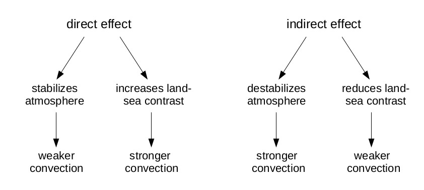
Putting these together, the direct and indirect effects have two opposing impacts on convection, and hence on summer stationary waves: they have the opposite effect on land-sea contrasts, and the opposite effect on atmospheric stability. These two impacts also oppose each other: the direct effect increases land-sea contrast (leading to stronger convection), while also stabilizing the atmosphere (which weakens convection), and vice versa for the indirect effect:

Looking at the plots of \(\theta_E\), there also seem to be important regional effects that aren’t explained by either of these, like the strong dipole in warming/cooling along the border of the Sahara and the Sahel, which extends over the Arabian peninsula. Another potentially important (and related) impact is differences in how the ITCZ responds to the direct and indirect effects. The ITCZ will shift north in response to the direct effect, since the northern hemisphere has more land and hence warms up more. But this won’t necessarily be canceled out by the indirect effect, since the land is still free to respond when SSTs increase. It’s unclear how to relate zonal-mean ITCZ shifts to the regional-scale, but we know these shifts would affect the patterns of convection.

So the stationary wave responses to the direct and indirect effects are complicated, and there probably isn’t a single explanation for how the summer stationary wave pattern changes.