This is a follow-up to my post "What Drives Uncertainty in Transient Warming?", which summarized a recent paper with Max Popp on "Probing the Sources of Uncertainty in Transient Warming on Different Time Scales". Here I’m going to provide some details on the analysis (A Jupyter notebook is also available here).

Theory

To understand the sensitivities of transient warming we started by thinking about the two box model I introduced in part 1. This can be solved for \(T_1\), either in real space or (more simply) by transforming to frequency space to give: $$ \hat{T_1} = \frac{1}{70\omega}\times \frac{F}{\lambda + ic\omega +\epsilon\gamma \left(1 - \gamma /(ic_0\omega + \gamma)\right)}, $$ where \(\omega\) is frequency and we assume CO\(_2\) concentrations are going up by 1% per year. Looking at this expression gives a first sense for why the forcing matters so much: it’s the only term in the numerator, whereas there are several terms in the denominator. So, for example, even if the climate feedback (\(\lambda\)) was zero, and the ECS was infinite, the transient warming would still be finite.

We then calculated the absolute value of \(\hat{T_1}\), which is a complicated expression, but can be simplified into four transient warming regimes (to make things more intuitive I'm going to move back to the time domain):

• the ultra-fast regime (\(t <\ t_H = c/(\lambda + \epsilon\gamma)\) ),
• the fast regime (\(t_H <\ t <\ <\ t_L= c_0 /\gamma\) ),
• the intermediate regime (\(t \leq t_L\) ),
• the slow regime (\(t > t_L\)).

Using ensemble-mean values from CMIP5, the fast time-scale \(t_H \approx\) 4 years and the slow time-scale \(t_L \approx\) 160 years. The fast and intermediate regimes are separated by the time it takes for the deep ocean to warm up significantly – when \(T_2\) is meaningfully greater than 0. Defining this as the time when \(t = 0.1 c_0 / \gamma\) gives a time-scale of 16 years.

Going through the different regimes: In the ultra-fast regime most of the uncertainty comes from the upper-ocean heat capacity \(c\). Basically, how quickly does the surface start warming up? If \(c\) is large then the warming in the first few years will be small, whereas if \(c\) is small then \(T_1\) will warm up quickly.

In the fast regime the forcing is responsible for most of the uncertainty, with \(\lambda\), \(\gamma\) and \(\epsilon\) also contributing. But because these are all in the denominator, their uncertainties partially cancel, and \(F\) is the leading source of uncertainty. On these time-scales \(c\) is small compared to \(λ + \epsilon \gamma\), so we don’t have to worry about the upper ocean heat capacity anymore.

Once the deep ocean has started warming, the ocean heat uptake parameters \(\gamma\) and \(\epsilon\) contribute less to uncertainty. You can see in the denominator of the equation that the term in brackets starts decreasing as \(c_0 \omega\) increases, and the effects of uncertainty in \(\gamma\) and \(\epsilon\) are muted. Physically, heat is transferred to the deep ocean through the term \(H = \epsilon\gamma(T_1 – T_2)\). \(H\) cools \(T_1\), and so \(\gamma\) and \(\epsilon\) damp transient warming. But as the two layers come into equilibrium \(T_1 – T_2\) becomes small, so \(H\) is also small, and \(\gamma\) and \(\epsilon\) matter less. In equilibrium \(H\) is zero, and it doens't matter what the values of \(\gamma\) and \(\epsilon\) are.

An interesting subtlety is that \(\gamma\) cools the surface layer directly, but also warms it indirectly by making \(T_2\) larger (and hence \(H\) smaller). These opposing direct and indirect effects on surface temperature mean that \(\gamma\) is responsible for less uncertainty than \(\epsilon\), which always damps surface temperature. (Note: one of the original motivations for our study was trying to clarify how the ocean contributes to transient warming uncertainty.)

Finally on long time-scales the two layers are in equilibrium with each other and we’re basically left with the ECS expression \(F / \lambda\), and the forcing and the feedback matter roughly equally.

So we can expect transient warming’s sensitivity to evolve as follows:

• for the first few years the upper ocean heat capacity matters most, but the importance of this quickly decreases,
• then the warming is most sensitive to the forcing, with the climate feedback and the ocean heat uptake terms (\(\gamma\) and \(\epsilon\)) also contributing,
• once the deep ocean has started heating up the sensitivity to the ocean heat uptake terms decreases, with the importance of \(\gamma\) decreasing faster than \(\epsilon\).

Through these different stages, the importance of the feedback \(\lambda\) relative to the forcing slowly increases, so that on the longest timescales transient warming is roughly as sensitive to \(\lambda\) as to \(F\).

CMIP5 data

To quantify things with some data, we fit the two box model to 1%/year simulations with a set of CMIP5 models. This gave the relative uncertainties in panel a of the figure below, where "relative uncertainty" is the standard deviation of a variable across the ensemble divided by the mean of the variable. Again, \(\lambda\) is about three times as uncertain as \(F\), though the most uncertain variable is actually \(c_0\).

To understand the contributions of each variable to uncertainty in the TCR, we then ran the two box model using the mean values of all the variables, except for one variable which we varied by \(\pm\) 2 standard deviations. E.g., we ran the model with \(F\), \(\lambda\), \(c\), \(c_0\) and \(\gamma\) set to their ensemble-mean values, but set \(\epsilon\) to one standard deviation above its ensemble-mean, to -2\(\times\) its standard deviation, etc. This gave the TCR estimates shown in the box-and-whisker plots of panel b. The largest spreads come when \(\lambda\) is varied and then when \(F\) is varied. \(\gamma\) and \(\epsilon\) are similar to each other, and the heat capacities are negligible.

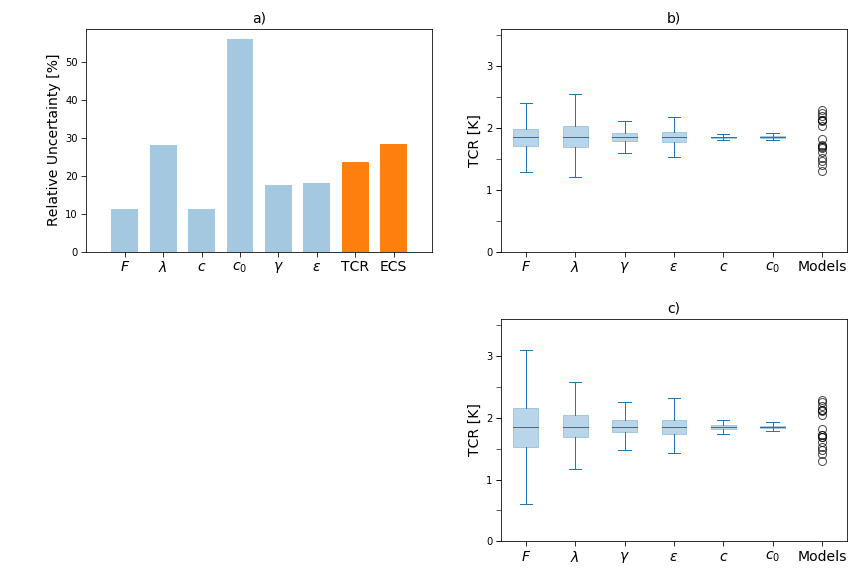
But this mixes the two aspects of uncertainty: the uncertainty in each variable, and the TCR’s sensitivity to that uncertainty. Varying \(\lambda\) produces the largest spread, but \(\lambda\) is also one of the most uncertain parameters. So we re-did the calculations but set the relative uncertainties for all variables to \(\lambda\)’s relative uncertainty (about 30%). These calculations (panel c) showed that the TCR is about twice as sensitive to uncertainty in the forcing as to uncertainty in the feedback, and suggested that if the forcing was as uncertain as the feedback our best guess for the TCR would be \(\sim\)0.5-3.5\(^\circ\)C, instead of the actual range of 1-2.5\(^\circ\)C.

We looked at how transient warming's sensitivies evolve over time by calculating the ratio \(r\) of the sensitivity of transient warming to uncertainty in each variable divided by the sensitivity of transient warming in the forcing \(F\). So if \(r_\gamma > 1\) at \(t =\) 20 years, it means that the warming after 20 years of increasing CO\(_2\) by 1%/year is more sensitive to uncertainty in \(\gamma\) than to uncertainty in \(F\). If \(r_\gamma <\ 1\), then the warming is more sensitive to \(F\) than to \(\gamma\).

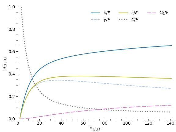
These calculations gave us exactly what we expected from the theory. Uncertainty in the upper ocean heat capacity matters a lot for the first few years, but quickly becomes negligible. The contributions of uncertainties in \(\gamma\) and \(\epsilon\) peak at around 20 years, then decrease as the deep ocean heats up, with the contribution from \(\gamma\) decreasing faster than the contribution from \(\epsilon\). And the feedback \(\lambda\) becoming more important over time (though even after 140 years \(r_F\) is only \(\sim\)0.7).

Toy Calculations

As mentioned in the previous post, Max and I discussed two implications of these results: (1) it’s dangerous to extrapolate from short-lived climate perturbations, like volcanic eruptions, to long-lived perturbations like CO\(_2\) increases, and (2) the feedbacks of models that are ‘tuned’ in some way to the historical record are strongly affected by historical forcing estimates.

We illustrated these implications with some toy calculations. First, we calculated the impulse response of the two-box model to a doubling of CO\(_2\). That is, we set \(F\) to \(F_{2XCO2}\) at year 1, and 0 at all other times. We did this calculation three times: once with the ensemble-mean parameters from the CMIP5 data, once with the upper ocean heat capacity \(c\) reduced by 25% and once with \(\lambda\) reduced by 25%. In the results (panel a) you can see that changing the heat capacity has a much larger effect on the response of the upper layer than changing \(\lambda\) – we’re in the ultra-fast regime – , with changing \(\lambda\) producing a pretty similar response to the "control" simulation. So if we were trying to fit the temperature response to a short-lived perturbation, like a volcanic eruption, we’d mostly be fitting the upper ocean heat capacity (and the volcanic forcing), and we wouldn't have to worry much about getting \(\lambda\) right.

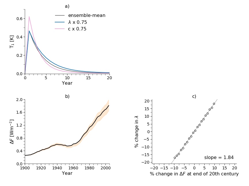
Our second toy calculation showed how the climate feedback of “tuned” models is strongly influenced by historical forcing estimates. We illustrated this through “historical” simulations of the 20th century with the two-box model, forcing it with an estimate of the total radiative forcing over the 20th century, \(\Delta F\) (panel b). We then varied the forcing by up to \(\pm\)1 standard deviation of \(F_{2XCO2}\) by setting \(\Delta F(t) = \Delta F(t) + \beta std(F_{2XCO2})\), with \(\beta\) varied from -1 to 1 in increments of 0.1. With this, we were trying to imitate how uncertainty in \(F_{2XCO2}\) would affect the estimated historical forcing.

For each forcing estimate, we set \(c\), \(c_0\), \(\lambda\) and \(\gamma\) to their ensemble-mean values and then searched for the value of \(\lambda\) that gave the best fit to the 20th temperature record. Panel c shows how the optimal value of \(\lambda\) varies as a function of the final forcing at the end of the 20th century (circles), with a linear least-squares regression giving that a 1% change in the net forcing results in a 1.84% change in the optimal value of \(\lambda\).

This calculation ignores things like the different forcing efficacies of greenhouse gases, the historical aerosol forcing and internal variability, but shows how sensitive the climate feedback in models that are tuned by fitting to the historical temperature record is to assumptions about the forcing over the 20th century. If you believe our toy calculations, then tuning the same model twice using historical forcing estimates that differed by 20% would give values of \(\lambda\) that differed by 37%.