An important result coming out of recent climate sensitivity studies is that the rate of global-mean warming depends on the spatial pattern of warming. There are different ways of interpreting this, but basically, different regions radiate to space more or less efficiently so that, for instance, if the warming is concentrated in a region which doesn’t emit strongly to space, global-mean warming is enhanced. Together, this is called the “pattern effect” (see more here and here).

Given the importance of the pattern of warming, it’s concerning then that climate models consistently get the pattern in the tropical Pacific wrong. In particular, historical simulations consistently predict that the east Pacific should have warmed, when observations show it cooling. This is a problem because the gradient of warming across the Pacific has been suggested as a key part of the net pattern effect (see here for example). Explaining why the models get this wrong, fixing this issue and understanding how this discrepancy might affect the relationship between observed and model climate sensitivity seem like some of the most important questions in climate science.

There are some papers looking into why the east Pacific is cooling and why models get it wrong. I'd had some trouble putting these together until I read a nice recent paper by Heede, Federov and Burls. Heede et al investigated changes in the Walker circulation in climate models, showing that the Walker circulation initially strengthens in response to increased CO\(_2\), then weakens, so that when the model finally equilibrates the Walker circulation is weaker than in the control state.

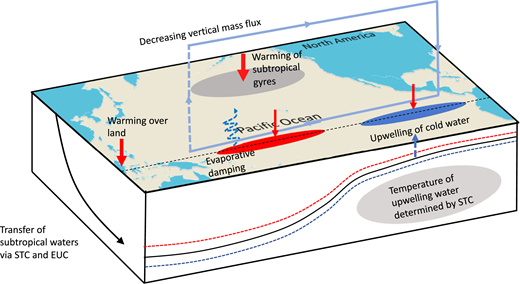
Heede et al mostly focused on the roles of two ocean mechanisms in driving this response. First, the "ocean thermostat" increases the zonal SST gradient across the Pacific, causing the Walker circulation to strengthen. This mechanism refers to the fact that the west Pacific warms up initially, but the warming in the east Pacific is delayed, because the SSTs there are mostly set by upwelling waters. Since it takes a while for these waters to warm up, the upwelling keeps the east Pacific cool for the first few decades of CO\(_2\) increase. But the waters in the subtropical gyres warm up, subduct and then upwell in the east Pacific, so that eventually the upwelling does feel the CO\(_2\) increase. This pathway is the "oceanic bridge", which reduces the SST gradient and weakens the Walker circulation. You can see these mechanisms in this nice schematic from Heede et al:

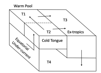
As shown in the paper, a simple model of the Pacific ocean which includes these effects qualitatively reproduces the behavior of climate models. The model consists of four boxes: an east Pacific box, a west Pacific box, a deep ocean box and a subtropical box (see schematic below). The equations for the temperature in each box are: $$ m_1 \frac{dT_1}{dt} = m_1H_1 + q(1 - \epsilon)(T_2 - T_1), $$ $$ m_2 \frac{dT_2}{dt} = m_2H_2 + q(T_4 - T_2), $$ $$ m_3 \frac{dT_3}{dt} = m_3H_3 + q\epsilon(T_2 - T_3) + q(1 - \epsilon)(T_1 - T_3), $$ $$ m_4 \frac{dT_4}{dt} = q(T_3 - T_4), $$ where \(T_i\) is the temperature in each box and \(m_i\) is the mass of each box. \(\epsilon\) is a branching parameter, which determines the ratio of water flowing out from the eastern and western tropical boxes, respectively. \(H_i\) is the temperature tendency induced by ocean-atmosphere heat fluxes and radiation: $$ H_i = \frac{1}{c_p\rho h_i} \left(H_{SW} - H_{LW} - H_{latent} - H_{sensible}\right). $$ Finally, \(q\) is the net upwelling, parameterized by $$ q = A_H(T_{eq} - T_3) + A_W(T_1 - T_2), $$ where \(A_H\) and \(A_W\) are "coupling parameters" for the Hadley and Walker circulations, and \(T_{eq}\) is the average temperature of the two boxes.

To understand the different mechanisms, we can look at the response of the temperatures in the two tropical Pacific boxes to an external forcing, keeping only first-order terms and assuming the masses and \(\epsilon\) are fixed:

\(m_1 \frac{d \Delta T_1}{dt} = F + m_1\Delta H_1 + q(1 - \epsilon)(\Delta T_2 - \Delta T_1) + \Delta q(T_2 - T_1)\) \(m_2 \frac{d \Delta T_2}{dt} = F + m_2\Delta H_2 + q(\Delta T_4 - \Delta T_2) + \Delta q(T_4 - T_2),\)

If we simplify by setting the masses of the two boxes equal: $$ \frac{d(\Delta T_1 - \Delta T_2)}{dt} = \frac{q(1 - \epsilon)}{m}(\Delta T_2 - \Delta T_1) + \frac{\Delta q}{m}(T_2 - T_1) - \frac{q}{m}(\Delta T_4 - \Delta T_2) - \frac{\Delta q}{m}(T_4 - T_2) + \Delta H_1 - \Delta H_2. $$

Initially, the first two terms on the right hand side are negative (\(\Delta T_2 - \Delta T_1 < 0\) and \(T_2 - T_1 < 0\)), while terms three and four are positive (we'll get to the fifth term in a moment). The ocean thermostat mechanism says that the sum of the four terms is positive, because \(T_4 – T_2 < T_2 – T_1\); the difference between the surface waters and the deep waters is larger than the difference across the Pacific, and because \(\Delta T_4 - \Delta T_2 \approx -\Delta T_2 < \Delta T_2 - \Delta T_1\) (it takes a while for the deep ocean to warm up). Hence \(\frac{d(\Delta T_1 - \Delta T_2)}{dt}\) is positive, and the SST gradient increases.

But as the surface gradient increases, \(\Delta T_2 - \Delta T_1\) gets larger (becomes more negative), and the ocean thermostat is self-limiting. Furthermore, the deep ocean starts warming up, via the oceanic bridge, so that eventually \(\Delta T_2 - \Delta T_4 < \Delta T_2 - \Delta T_1\). The SST difference starts decreasing, until it ends up being smaller than in the control climate.

This is how the tropical Pacific behaves in climate models when CO\(_2\) concentrations are increased. But we can also use the box model to understand discrepancies between models and obs. For instance, Seager et al suggested that the problem in models is that the relative humidity is too high and the winds are too weak over the East Pacific. This means that \(\Delta H_2\) is too small (because the latend heat flux -- \(H_{latent}\) -- is too small). In reality, the lower relative humidity and stronger winds have produced cooling via evaporation in the east Pacific, causing \(\Delta H_2\) to be larger in observations than in models (\(\Delta H_{2, obs}\) < \(\Delta H_{2, models}\) < 0). (Note: I couldn't find any plots of evaporation in Seager et al). As you can see from the model equations, this would cool the eastern Pacific, and increase the SST gradient across the Pacific.

In a different take, Karnauskas and Coats attributed things to the equatorial undercurrent, claiming that this has strengthened recently. In the context of the model above, this means \(\Delta q\) has increased more in reality than in models, which would cause \(\Delta T_1 - \Delta T_2\) to increase faster, or \(T_2\) to cool. Karnauskas and Coats showed that the strength of the equatorial undercurrent is biased in models compared to an ocean reanalysis, and so the models have trouble capturing this effect.

In either case, biases in the surface winds seem to be at least partly responsible for the warming in the east Pacific in models (Karnauskas and Coats find that part of the bias in the equatorial undercurrent comes from biases in the surface winds). This seems like it might be quite hard to fix, since the winds in the deep tropics are related to global-scale energy imbalances. It would be interesting to run simulations with a model in which the winds over the equatorial Pacific are nudged to a stronger mean state, to see how this affects the (transient and equilibrium) climate sensitivity. Another thing I worry about is whether the discrepancy in east Pacific warming affects emergent constraints based on tropical cloud variability, which often involve variability over the east Pacific. If models are getting the long-term trend in this region wrong, maybe they are getting the link between variability and the forced response wrong?